Understanding buzzdetect model metrics
buzzdetect core
Overview
There are a few pieces of jargon we often use when referring to the performance of our buzzdetect models. Fortunately, the tests of our models are fairly straightforward. In this post, we’ll do a deep dive on our terminology and look at some of the behaviors and implications of the model metrics.
So far, we treat our models as simple binary predictors. Is there buzzing in the frame or not? The models can’t (yet) identify the insect producing the buzz and, while they’ve technically been trained to detect other events like rain and passing cars, we only include those events in the training dataset to improve performance on bees and haven’t tested model performance on non-buzz events.
Treating results as binary trials, there are three resulting measures of model performance that we refer to as the model metrics: sensitivity, precision, and false positive rate. These interrelated values are themselves functions of the threshold applied to the activation value for the buzz neuron of the model. Let’s define all five terms.
TL;DR
Sensitivity is the probability that we get a detection given that a frame contains a buzz.
Precision is the probability that there is a buzz given that there was a detection.
False positive rate is the probability that a non-buzz frame produces a detection.
The threshold is the activation value above which we call a detection.
The activation value is the score given by the output neuron trained to detect buzzes.
Activation and Thresholds
Every row in a buzzdetect result file represents one frame, one discrete portion of audio that was fed into the model. Every column (except the “start” column) represents a different type of audio event the model has been trained to classify, with values corresponding to those neurons’ activations: the numerical output of the neural network for that neuron. The model is a huge pile of math; the activations are the outputs of that pile given the input audio. The activation value is a bit abstract. We don’t make any modification of the activations, though other tools do. BirdNET rescales activations with a sigmoid function to bound them between zero and one (see Wood and Kahl 2024). This does tidy up the values, but it doesn’t really change how they’re used or what they mean. We could try to map the activations to a probability (and we do, later in this post), but this mapping is context-dependent. We don’t want to imply that a given activation value implies a fixed chance of a buzz, so buzzdetect outputs the unmodified activation values.
To turn activations into detections, the user must apply a threshold. This is simply a number that sets the lower limit for a detection. When activation > threshold, a detection is called. The choice of a threshold depends on the signal-to-noise ratio of the underlying data. Sites with a high amount of pollinator activity will show obvious trends even under very strict thresholds. Thresholding buzzdetect results is handled by our buzzr package.
The metrics: sensitivity, precision, and false positive rate
Applying a threshold turns our continuous activations into discrete detections. The frame could be in any one of four states: true positive (a detection is called and a buzz really is present), false positive (a detection is called, but there was no buzz), true negative (no detection, no buzz), or false negative (a buzz was missed). This is where our metrics come in:
False positive rate, \(P(\text{detection}|\text{non-buzz})\), is simply the probability that a non-buzz frame produces a detection. Given a lot of non-buzz audio, how often does the model think there’s a buzz?
Sensitivity, \(P(\text{detection}|\text{buzz})\), is the probability that we get a detection given that a frame contains a buzz. Given a lot of buzzing audio, how often does the model correctly pick up the buzzing?
Precision, \(P(\text{buzz}|\text{detection})\), is a little less straightforward. It’s the probability that there really is a buzz in the audio given that we see a detection. This might sound similar to false positive rate and the probability calculation is just sensitivity in reverse, but precision is very much a distinct concept. It’s easiest to think of it as a signal:noise ratio. Precision is a joint function of the other two metrics and of the amount of buzzes in the audio.
It’s a function of false positive rate because the more likely we are to have false positives, the less confident we are that there will really be a buzz when we see a detection.
It’s a function of sensitivity because the more likely we are to pick up on true buzzes, the more confident we can be in our detections.
It’s a function of the amount of buzzes because more buzzing means more chances for true positives and fewer chances for false positives. Imagine a model that inherently has a 5% false positive rate and 50% sensitivity. If we applied this model to 100 frames of audio where 80 contain buzzes and 20 do not, we would expect to see
0.5×80 = 40true positive frames and0.05×20 = 1false positive frame, a precision of40/41 = 98%. If we applied the same model to different audio containing 20 buzz frames and 80 non-buzz frames, we would expect to see0.5×20 = 10true positive frames and0.05×80 = 4false positive frames, a precision of10/14 = 71%.
In a way, precision is the metric to be concerned about. Who cares how sensitive you are if you’re getting a lot of noise with that signal? What does it matter how low the false positive rate is if you can’t detect any bees in the first place? Or, in the other direction, maybe you could tolerate more false positives because in return you would get so many more true positives! Precision offers a balancing point between false positives and false negatives, informed by the real world rate of buzzes. For this reason, we shoot for a threshold that corresponds to 95% precision.
Metrics across the thresholds
Let’s graph how these metrics relate to one another as we move across threshold values. We’ll use the data from our tests on model_general_v3. These data are available in the Zenodo repository for the buzzdetect manuscript. Read the manuscript to see how these data were created. The full code to reproduce these metrics is also in the repository.
Let’s plot the entire range of activations seen during model testing. This plot is interactive, try moving your cursor across it to see the values change.
Precision can’t be lower than ~17%, because that was the background rate of buzzing in our audio. If you just call everything a buzz, you’ll still be right 17% of the time.
- Note that the test audio were only from daytime hours. The precision would be lower if we had included all of the nighttime audio.
Precision hits nearly 100% at a threshold of -0.7. There’s no point in cranking your threshold any higher.
Even a small increase in false positive rate can tank precision. 0.2% → 0.7% in false positive rate might not seem like much, but it drops precision from 99% to 90%. There’s a lot more non-buzz audio than there is buzz audio - false positives really matter!
This graph covers all observed activation values of the buzz neuron. That’s a ridiculous extent when we’re suggesting using thresholds at 95% or higher precision. Let’s zoom in and graph things differently; let’s look at the trade-off between our reasonable range of precision values and our other two metrics.
Trading off metrics
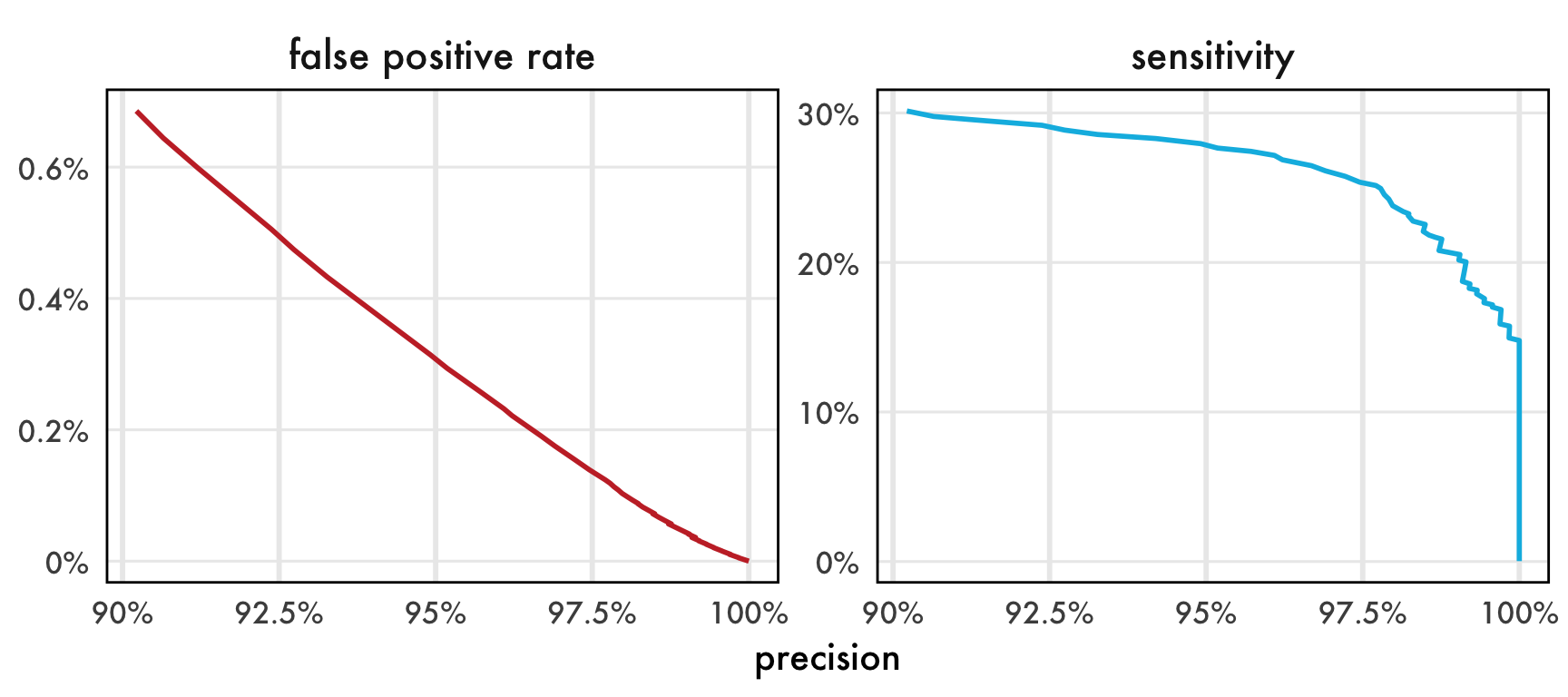
We find that thresholds are prone to producing false positives (and sometimes systematic ones, e.g. peaks instead of uniform noise) at less than 95% precision on our test set. This means that the maximum useful sensitivity value is ~30%. While we’d love to train a perfectly sensitive model, we think that this level of sensitivity is still perfectly acceptable for most analyses. 30% applied across every second of the day is a lot of detections. Hundreds to thousands! Include the high-replication enabled by passive monitoring and the signal to noise ratio is quite strong. We’ve also found that analyses give remarkably similar results are extraordinarily high thresholds. And, hey, what’s the sensitivity of a sweep net, anyways?
We can see that sensitivity stays relatively constant until it hits a wall shortly after 97.5%.
- This trend is actually expected because, in the activation space, the distance between 97.5% and 100% precision is much larger than that from 90% to 97.5%.
- The steeper falloff in false positive rate seems to suggest that signal:noise is maximized where the two curves are most divergent, around 97.5%.
False positive rate is very well behaved (less jagged) as precision increases. This may just be because there are a lot more frames of non-buzz audio from which to calculate FPR.
References
Wood, Connor M., and Stefan Kahl. 2024. “Guidelines for Appropriate Use of BirdNET Scores and Other Detector Outputs.” Journal of Ornithology 165 (3): 777–82. https://doi.org/10.1007/s10336-024-02144-5.