Strange sounds of the field, an investigation with SeeNote

It was a surprise, early in my bioacoustics career, to learn that the world is full of sound. Maybe that’s obvious to everyone else, but I would have said the depths of a soybean field doesn’t sound like much. And that’s not a naive guess, I’ve been deep in many soybean fields! I remember seeing little beetles chewing hole punches out of soybean leaves, I remember feeling the cracked clay under my feet, and I guess I remember hearing the swish of the plants as I sifted through the rows, but I don’t remember hearing much else.

Now I’m constantly listening to audio from all sorts of places for my research. Sometimes it’s to make training data for buzzdetect and other times I’m digging into the bioacoustic results to listen for myself. The combination of concerted attention and using spectrograms to visualize the sound reveals so much that our brains filter out of our experience. Birds calling, frogs chirping, crickets trilling, planes, trains, and automobiles - all these things can be shrouded in some sort of attention-cloak. I’ve found myself annotating an audio file thinking there’s nothing going on, only to realize on second listen that there’s a whole chorus of sound that my brain dismissed as “background” on my behalf.

Then, there are sounds that are very much in the foreground. Here’s the story of how I accidentally eavesdropped on the amorous evening of a pair of hoverflies.

Part One: false positives

False positives are, unfortunately, an unavoidable part of passive monitoring. The models that ship with buzzdetect v2 are extraordinarily good, compared to the model we published with, anyways. Many of the sounds that produced systematic false positives with the old model are easily handled by the new ones, in part because we have a “hard negatives” training arm where we do targeted annotation of false positives to add them to the training set. But, still, there will always be new sounds you haven’t encountered before. So, I still routinely check my buzzdetect results against the raw audio, even just to get a better sense of the ground truth.

At the time of writing this post, I haven’t made a good walkthrough for all the new features in SeeNote - it’s come a very long way since initial release! This post will have to serve as a demo of my workflow for bioacoustics and how it’s been supercharged by SeeNote.

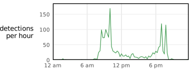
I did some work this summer in a zucchini plot. Zucchini being a cucurbit, the flowers are all closed by midday. So, we don’t expect to see any pollinator activity in the plots after, say, 12:00pm. Imagine my surprise when I see the following plot:

library(dplyr)
library(ggplot2)

results <- buzzr::bin_directory(
  dir_results,
  thresholds = c(
    ins_buzz=0.0,
    ambient_rain=0,
    human=0,
    mech_auto=0,
    mech_plane=0
  ),
  posix_formats = '%y%m%d_%H%M',
  tz = 'America/New_York',
  dir_nesting = c('date_deployed', 'recorder'),
  binwidth=15,
  workers=8,
  calculate_rate = T
)  %>% 
  filter(lubridate::date(bin_datetime) == '2026-06-24')

ggplot(
  results %>% 
    # the results have multiple recorders on this date, we'll average them together
    group_by(bin_datetime) %>% 
    buzzr::summarize_detections(),
  aes(
    # time of day the bin starts
    x = bin_datetime,

    # detectionrate can be a bit obscure; I like plotting "detections per hour".
    # we can get that by multiplying our detection rate by the number of frames in an hour
    y = detectionrate_ins_buzz * buzzr::frames_expected(60, 0.96)
  )
) +
  geom_path(color = '#4DA25C') +
  buzzr::theme_buzzr() +
  ylab('detections\nper hour') +

  # ggplot adds space around your data's extent. It can be pretty annoying. We'll mostly undo it.
  # x axis will go edge-to-edge
  scale_x_datetime(labels=buzzr::label_hour(), expand=0) +
  
  # y axis will hit 0 right at the bottom, but we'll give 10% headroom
  scale_y_continuous(expand=expansion(c(0, 0.1))) +
  theme(axis.title.x = element_blank())

This analysis was run with the new heavy_v1 model. I thought I solved these false positives! Let’s use SeeNote to investigate what’s going on.

Part Two: looking closer

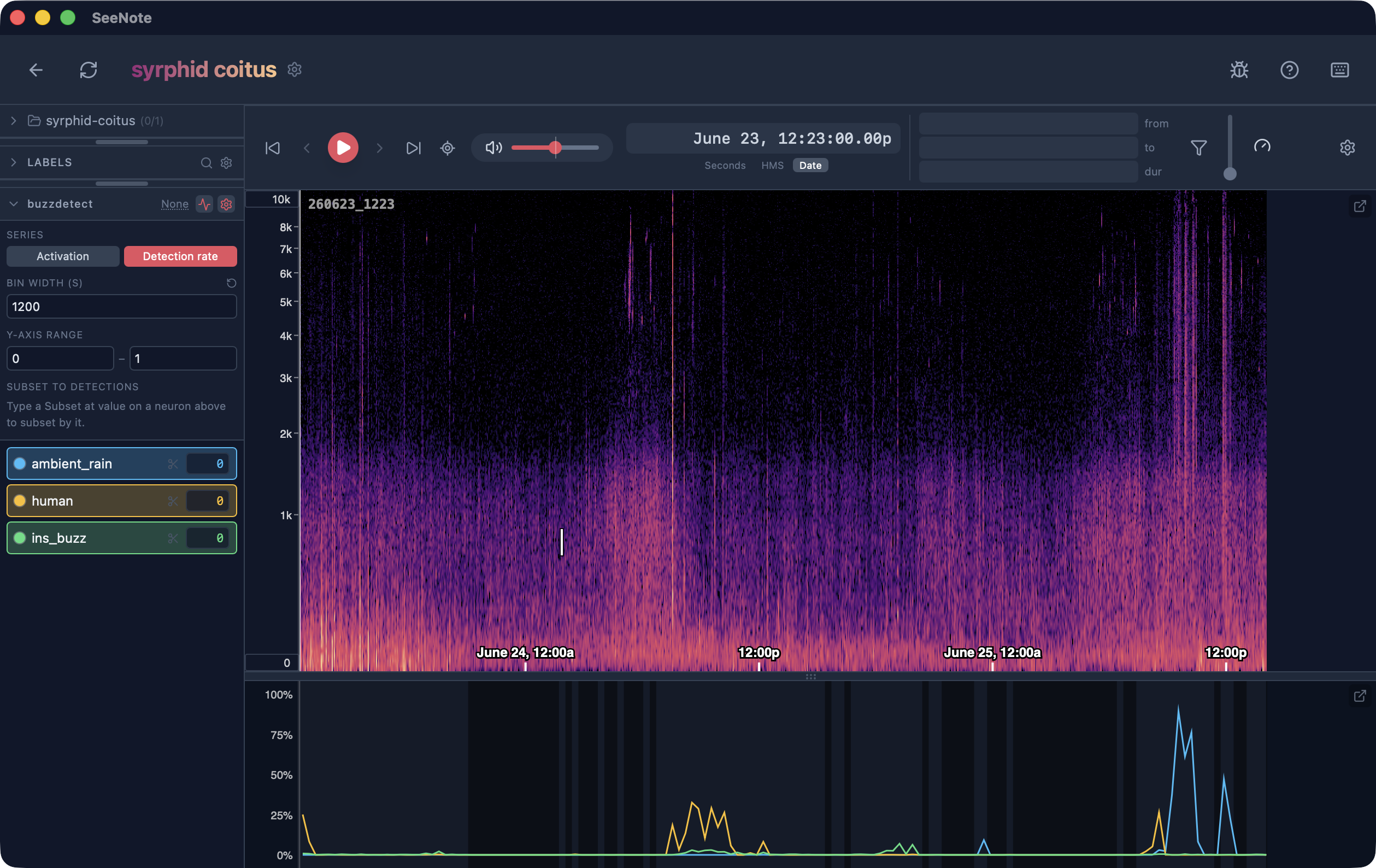
I’ll pick the recorder that had the largest evening spike of detections. The audio file spans three days; here’s the zoomed out view:

Already, we see a few things:

• The orange trace is the “human” neuron, detecting speech. There are three spikes of activity; the first is me setting up the microphones, the second is me returning to the site and instructing an undergrad on data collection, the third is other researchers working at the site.

  • This touches on a point I’ve been chewing on a lot lately. Passive monitoring raises some privacy concerns - some of our work has happened in spaces where people are having conversations they may not want to be on record. Even when standing in a field of dozens of active microphones, I’ve had discussions with site owners that I’m quite certain they would not want to be publicized! On the other hand, sharing data openly is good for the advancement of bioacoustics. Since the latest models detect human speech very reliably, it should be easy to write up a little script that blanks out frames positive for speech, sanitizing the data for public sharing. If I ever get around to making that, I’ll share it on the blog.

• The blue trace is the “rain” neuron. Sure enough, June 25 was a rainy morning! It’s extremely valuable to get this weather data for free - my datasets cover so many days and sites, it would be a pain to try to infer rain from the nearest weather stations for each site.

• The green trace is the insect flight buzz neuron. We can see our late-evening spike towards the middle, but it’s drowned out by the other results because there are comparatively few buzzes. Let’s drop the other neurons and zoom in.

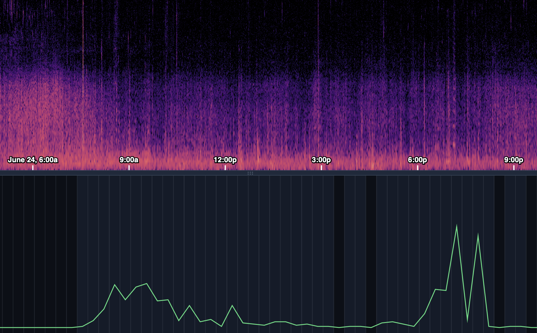
Sure enough, we get our trend back. It’s a little different than our first graph since this is just one recorder. In fact, there’s a higher detection rate in the evening than in the morning! What’s going on here? Even at this zoom level, my eyes see something intriguing in the spectrogram right at that spike. In fact, it looks like a buzz…

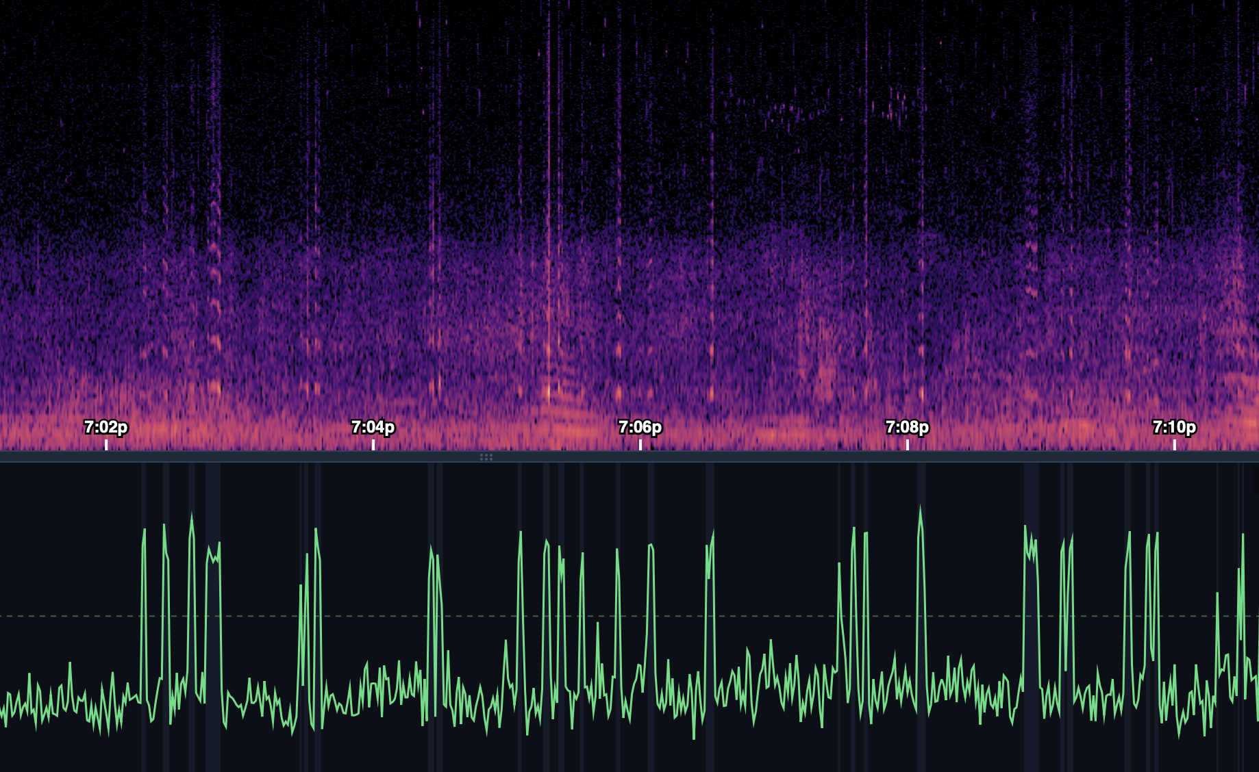
Enhance!

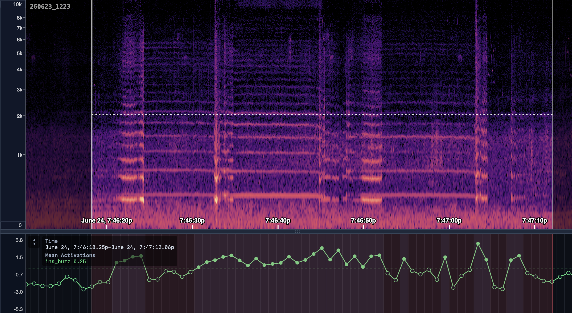
How’s that for a trend? I’m now plotting per-frame neuron activations instead of binned detection rates. We see numerous individual, well-separated spikes. The baseline neuron activation is -3, the peaks are ~2.5. Given that we call buzzes at 0 and I usually nudge the threshold by ~0.25 for one step up, the model is very confident that these are buzzes. Let’s listen to one.

Part Three: true positives!

What on earth is this? It sounds to be two buzzes, both higher-pitched than honey bees, one lower and intermittent, one higher and steady. They change together, but sound like two distinct animals. The speed with which they take off makes me think something small bodied. Hmmm….

It would appear we’ve accidentally snooped on the evening recreation of a couple of hoverflies. These aren’t false positives at all - at least, from the model’s perspective. I suppose it’s a different kind of false positive. We got the right answer to our question (there really were buzzes at 8:00pm), but we didn’t ask the question we thought we were asking (“when is pollination carried out in this crop?”). This is why reliably discriminating between species, à la BirdNet, is the holy grail of insect bioacoustics right now.

I haven’t listened to all of the recordings, but across a few weeks of intermittent monitoring, I don’t see another day that has a similar spike of detections in the evening. On this day, however, most of our microphones showed the same trend in the small zucchini plot. Is syrphid mating so constrained in time? Cued by some environmental factors? We’re sitting on a huge library of field recordings - could there be an interesting study in training a model to detect hoverfly mating and checking against our library? If there are any hoverfly experts out there, get in touch!

Wrapping up

The world is full of sound. I routinely hear strange and novel noises in our field recordings. It’s fun to listen - something about sound is uniquely transportative. Sometimes I start investigating a field recording and accidentally leave it running in the background because I forget that my office ambiance isn’t actually a zucchini field at dusk. If I notice, I usually leave it running anyways.

Hopefully this post also serves as a demo for the ways that SeeNote can let you get more out of your data! I’m finding it an invaluable tool as I build my analyses; there’s a wonderful feeling of frictionlessness in the whole pipeline now that I’ve gotten it a little more fleshed out. Set out the recorders, offload the files with FileSync, pass them through buzzdetect, wrangle and plot them with buzzr, tune the analysis and delve into the results with SeeNote. Hey, maybe building out all of these tools really was the right decision instead of writing my dissertation!

Edit: bonus round! Some real false positives

Mere minutes after posting this, I noticed some systematic false positives in one of my deployments. In this case, the spike was seen in all recorders at the site, which can be indicative of some distant, loud sound that’s producing the positives.

Following this same workflow, I look and see:

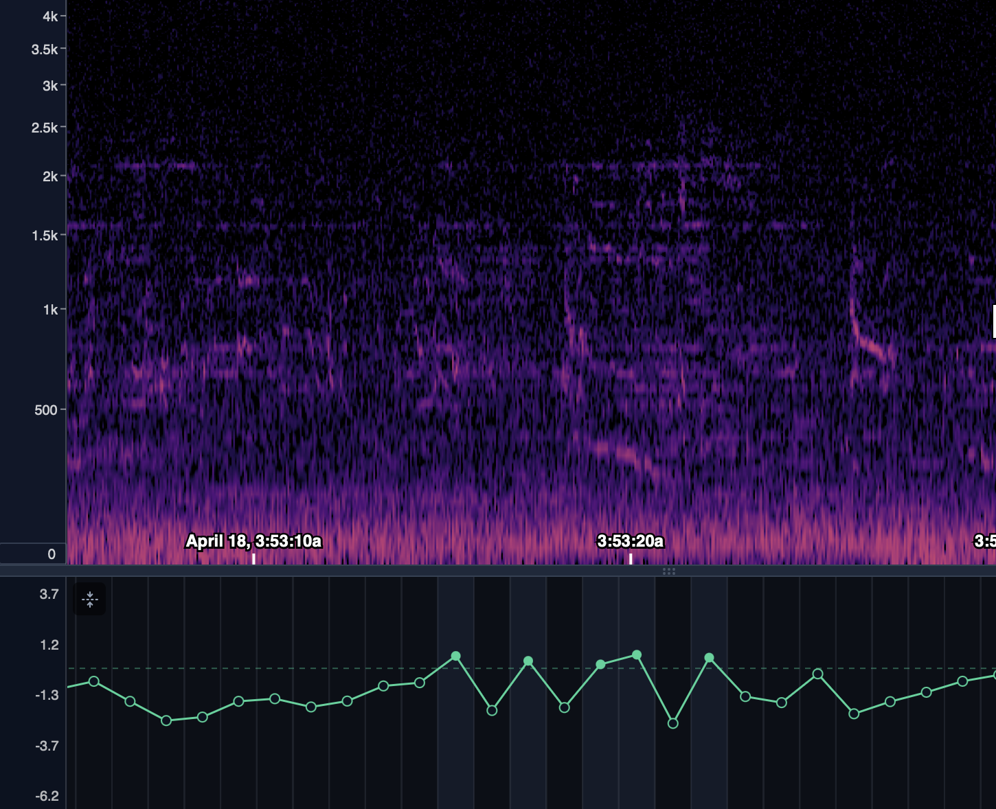
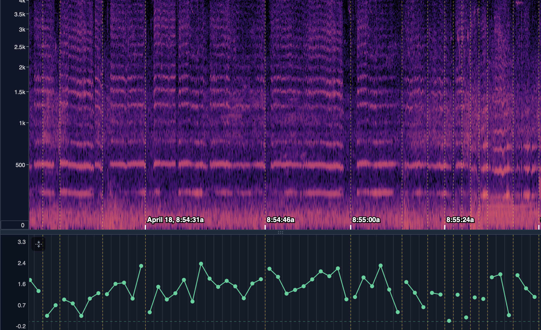
Definitely not buzzes! In this case it seems to be…a house party at 4:00am? There’s music, a dog barking, and people talking. Absolutelly none of this sounds remotely like a bee buzz, and all of it is represented in the training set! But sometimes the underlying acoustic context - quiet, nighttime, no birds - seems to shift the audio into a space the model has never seen before that must overlap with the learned features from buzzes. Sometimes, model training feels like sonic whack-a-mole. How could we have known we need to captures samples of a 4:00am house party!? These issues are relatively rare - this experiment covers 8 sites and 57 recording dates for ~15,000 hours of recording. This is the only occurrence of false positives that I’m aware of in the experiment, and I could filter it out with a threshold of 1, which would still leave plenty of headroom for loud, strong buzzes:

Still, annoying!